")
Feature Scaling is a technique to standardize the independent features present in the data in a fixed range. It is performed during the data pre-processing.
Working:
Given a data-set with features- No of years lived, Income, Location with the data size of 5000 people, each having these independent data features.
Each data point is labeled as:
• Class1- YES (means with the given No of years lived, Income, Location feature value one can buy the property)
• Class2- NO (means with the given No of years lived, Income, Location feature value one can’t buy the property).
Using dataset to train the model, one aims to build a model that can predict whether one can buy a property or not with given feature values.
Once the model is trained, an N-dimensional (where N is the no. of features present in the dataset) graph with data points from the given dataset, can be created. The figure given below is an ideal representation of the model.
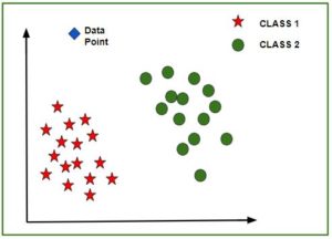
As shown in the figure, star data points belong to Class1 – Yes and circles represent Class2 – No labels and the model gets trained using these data points. Now a new data point (diamond as shown in the figure) is given and it has different independent values for the 3 features (No of years lived, Income, Location) mentioned above. The model has to predict whether this data point belongs to Yes or No.
Prediction of the class of new data point:
The model calculates the distance of this data point from the centroid of each class group. Finally this data point will belong to that class, which will have a minimum centroid distance from it.
The distance can be calculated between centroid and data point using these methods-
• Euclidean Distance : It is the square-root of the sum of squares of differences between the coordinates (feature values – No of years lived, Income, Location) of data point and centroid of each class. This formula is given by Pythagorean theorem.
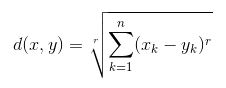
where x is Data Point value, y is Centroid value and k is no. of feature values, Example: given data set has k = 3
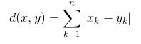
• Manhattan Distance : It is calculated as the sum of absolute differences between the coordinates (feature values) of data point and centroid of each class.
• Minkowski Distance : It is a generalization of above two methods. As shown in the figure, different values can be used for finding r.

Need of Feature Scaling:
The given data set contains 3 features – No of years lived, Income, Location. Consider a range of 10- 60 for No of years lived, 1 Lac- 40 Lacs for Income, 1- 5 for BHK of Flat. All these features are independent of each of other.
Suppose the centroid of class 1 is [40, 22 Lacs, 3] and data point to be predicted is [57, 33 Lacs, 2].
Using Manhattan Method,
Distance = (|(51 - 68)| + |(3300000 - 4400000)| + |(4 - 3)|)
It can be seen that Income feature will dominate all other features while predicting the class of the given data point and since all the features are independent of each other i.e. a person’s Income has no relation with his/her No of years lived or what requirement of flat he/she has. This means that the model will always predict wrong.
So, the simple solution to this problem is Feature Scaling. Feature Scaling Algorithms will scale No of years lived, Income, Location in fixed range say [-1, 1] or [0, 1]. And then no feature can dominate other.