Density Based Spatial Clustering of Applications with Noise(DBCSAN) is a clustering algorithm which was proposed in 1996. In 2014, the algorithm was awarded the ‘Test of Time’ award at the leading Data Mining conference, KDD.

Dataset – Credit Card.

Step 1: Importing the required libraries

import numpy as np
import pandas as pd
import matplotlib.pyplot as plt

from sklearn.cluster import DBSCAN
from sklearn.preprocessing import StandardScaler
from sklearn.preprocessing import normalize
from sklearn.decomposition import PCA
Step 2: Loading the data

X = pd.read_csv('..input_path/CC_GENERAL.csv')

# Dropping the CUST_ID column from the data
X = X.drop('CUST_ID', axis = 1)

# Handling the missing values
X.fillna(method ='ffill', inplace = True)

print(X.head())

Step 3: Preprocessing the data

# Scaling the data to bring all the attributes to a comparable level
scaler = StandardScaler()
X_scaled = scaler.fit_transform(X)

# Normalizing the data so that
# the data approximately follows a Gaussian distribution
X_normalized = normalize(X_scaled)

# Converting the numpy array into a pandas DataFrame
X_normalized = pd.DataFrame(X_normalized)
Step 4: Reducing the dimensionality of the data to make it visualizable

pca = PCA(n_components = 2)
X_principal = pca.fit_transform(X_normalized)
X_principal = pd.DataFrame(X_principal)
X_principal.columns = ['P1', 'P2']
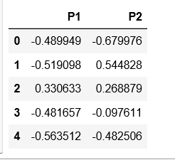
print(X_principal.head())

Step 5: Building the clustering model

# Numpy array of all the cluster labels assigned to each data point
db_default = DBSCAN(eps = 0.0375, min_samples = 3).fit(X_principal)
labels = db_default.labels_
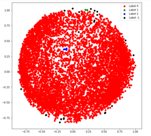
Step 6: Visualizing the clustering

# Building the label to colour mapping
colours = {}
colours[0] = 'r'
colours[1] = 'g'
colours[2] = 'b'
colours[-1] = 'k'

# Building the colour vector for each data point
cvec = [colours[label] for label in labels]

# For the construction of the legend of the plot
r = plt.scatter(X_principal['P1'], X_principal['P2'], color ='r');
g = plt.scatter(X_principal['P1'], X_principal['P2'], color ='g');
b = plt.scatter(X_principal['P1'], X_principal['P2'], color ='b');
k = plt.scatter(X_principal['P1'], X_principal['P2'], color ='k');

# Plotting P1 on the X-Axis and P2 on the Y-Axis
# according to the colour vector defined
plt.figure(figsize =(9, 9))
plt.scatter(X_principal['P1'], X_principal['P2'], c = cvec)

# Building the legend
plt.legend((r, g, b, k), ('Label 0', 'Label 1', 'Label 2', 'Label -1'))

plt.show()

Step 7: Tuning the parameters of the model

db = DBSCAN(eps = 0.0375, min_samples = 50).fit(X_principal)
labels1 = db.labels_
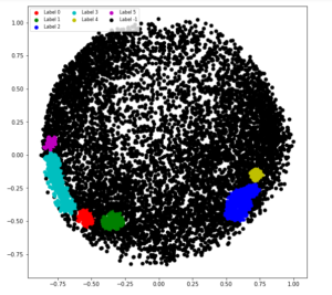
Step 8: Visualizing the changes

colours1 = {}
colours1[0] = 'r'
colours1[1] = 'g'
colours1[2] = 'b'
colours1[3] = 'c'
colours1[4] = 'y'
colours1[5] = 'm'
colours1[-1] = 'k'

cvec = [colours1[label] for label in labels]
colors = ['r', 'g', 'b', 'c', 'y', 'm', 'k' ]

r = plt.scatter(
X_principal['P1'], X_principal['P2'], marker ='o', color = colors[0])
g = plt.scatter(
X_principal['P1'], X_principal['P2'], marker ='o', color = colors[1])
b = plt.scatter(
X_principal['P1'], X_principal['P2'], marker ='o', color = colors[2])
c = plt.scatter(
X_principal['P1'], X_principal['P2'], marker ='o', color = colors[3])
y = plt.scatter(
X_principal['P1'], X_principal['P2'], marker ='o', color = colors[4])
m = plt.scatter(
X_principal['P1'], X_principal['P2'], marker ='o', color = colors[5])
k = plt.scatter(
X_principal['P1'], X_principal['P2'], marker ='o', color = colors[6])

plt.figure(figsize =(9, 9))
plt.scatter(X_principal['P1'], X_principal['P2'], c = cvec)
plt.legend((r, g, b, c, y, m, k),
('Label 0', 'Label 1', 'Label 2', 'Label 3 'Label 4',
'Label 5', 'Label -1'),
scatterpoints = 1,
loc ='upper left',
ncol = 3,
fontsize = 8)
plt.show()