")
Suppose there are set of data points that needs to be grouped into several parts or clusters based on their similarity. In machine learning, this is known as Clustering.
There are several methods available for clustering like:
- K Means Clustering
- Hierarchical Clustering
- Gaussian Mixture Models
etc.
In this article, Gaussian Mixture Model will be discussed.
Normal or Gaussian Distribution
In real life, many datasets can be modeled by Gaussian Distribution (Univariate or Multivariate). So it is quite natural and intuitive to assume that the clusters come from different Gaussian Distributions. Or in other words, it is tried to model the dataset as a mixture of several Gaussian Distributions. This is the core idea of this model.
In one dimension the probability density function of a Gaussian Distribution is given by
where $mu$ and $sigma^2$ are respectively mean and variance of the distribution.
For Multivariate ( let us say d-variate) Gaussian Distribution, the probability density function is given by
Here $mu$ is a d dimensional vector denoting the mean of the distribution and $Sigma$ is the d X d covariance matrix.
Gaussian Mixture Model
Suppose there are K clusters (For the sake of simplicity here it is assumed that the number of clusters is known and it is K). So mu and Sigma is also estimated for each k. Had it been only one distribution, they would have been estimated by maximum-likelihood method. But since there are K such clusters and the probability density is defined as a linear function of densities of all these K distributions, i.e.
where pi_k is the mixing coefficient for k-th distribution.
For estimating the parameters by maximum log-likelihood method, compute p(X|mu, Sigma, pi).
Now define a random variable gamma_k(X) such that gamma_k(X)=p(k|X).
From Bayes’theorem,
Now for the log likelihood function to be maximum, its derivative of p(X|mu, Sigma, pi) with respect to mu, Sigma and pi should be zero. So equaling the derivative of p(X|mu, Sigma, pi) with respect to mu to zero and rearranging the terms,
Similarly taking derivative with respect to Sigma and pi respectively, one can obtain the following expressions.
And
Note:  denotes the total number of sample points in the k-th cluster. Here it is assumed that there are total N number of samples and each sample containing d features are denoted by x_i.
So it can be clearly seen that the parameters cannot be estimated in closed form. This is where Expectation-Maximization algorithm is beneficial.
Expectation-Maximization (EM) Algorithm
The Expectation-Maximization (EM) algorithm is an iterative way to find maximum-likelihood estimates for model parameters when the data is incomplete or has some missing data points or has some hidden variables. EM chooses some random values for the missing data points and estimates a new set of data. These new values are then recursively used to estimate a better first data, by filling up missing points, until the values get fixed.
These are the two basic steps of the EM algorithm, namely E Step or Expectation Step or Estimation Step and M Step or Maximization Step.
Estimation step:
initialize mu_k, Sigma_k and pi_k by some random values, or by K means clustering results or by hierarchical clustering results.
Then for those given parameter values, estimate the value of the latent variables (i.e gamma_k)
Maximization Step:
Update the value of the parameters( i.e. mu_k, Sigma_k andpi_k) calculated using ML method.
Algorithm:
Initialize the mean mu_k,
the covariance matrix Sigma_k and
the mixing coefficients pi_k
by some random values. (or other values)
Compute the gamma_k values for all k.
Again Estimate all the parameters
using the current gamma_k values.
Compute log-likelihood function.
Put some convergence criterion
If the log-likelihood value converges to some value
( or if all the parameters converge to some values )
then stop,
else return to Step 2.
Example:
In this example, IRIS Dataset is taken. In Python there is a GaussianMixture class to implement GMM.
Note: This code might not run in an online compiler. Please use an offline ide.
- Load the iris dataset from datasets package. To keep things simple, take only first two columns (i.e sepal length and sepal width respectively).
- Now plot the dataset.
import numpy as np
import pandas as pd
import matplotlib.pyplot as plt
from pandas import DataFrame
from sklearn import datasets
from sklearn.mixture import GaussianMixture# load the iris dataset
iris = datasets.load_iris()# select first two columns
X = iris.data[:, :2]# turn it into a dataframe
d = pd.DataFrame(X)# plot the data
plt.scatter(d[0], d[1])

3. Now fit the data as a mixture of 3 Gaussians.
4. Then do the clustering, i.e assign a label to each observation. Also find the number of iterations needed for the log-likelihood function to converge and the converged log-likelihood value.
gmm = GaussianMixture(n_components = 3)
# Fit the GMM model for the dataset
# which expresses the dataset as a
# mixture of 3 Gaussian Distribution
gmm.fit(d)
# Assign a label to each sample
labels = gmm.predict(d)
d['labels']= labels
d0 = d[d['labels']== 0]
d1 = d[d['labels']== 1]
d2 = d[d['labels']== 2]
# plot three clusters in same plot
plt.scatter(d0[0], d0[1], c ='r')
plt.scatter(d1[0], d1[1], c ='yellow')
plt.scatter(d2[0], d2[1], c ='g')
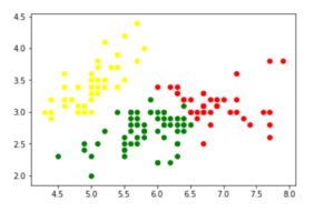
5. Print the converged log-likelihood value and no. of iterations needed for the model to converge
# print the converged log-likelihood value
print(gmm.lower_bound_)
# print the number of iterations needed
# for the log-likelihood value to converge
print(gmm.n_iter_)</div>
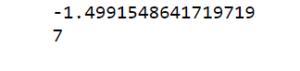
6. Hence, it needed 7 iterations for the log-likelihood to converge. If more iterations are performed, no appreciable change in the log-likelihood value, can be observed.