")
Problem with Simple Convolution Layers
- For a gray scale (n x n) image and (f x f) filter/kernel, the dimensions of the image resulting from a convolution operation is (n – f + 1) x (n – f + 1).
For example, for an (8 x 8) image and (3 x 3) filter, the output resulting after convolution operation would be of size (6 x 6). Thus, the image shrinks every time a convolution operation is performed. This places an upper limit to the number of times such an operation could be performed before the image reduces to nothing thereby precluding us from building deeper networks. - Also, the pixels on the corners and the edges are used much less than those in the middle.
For example,
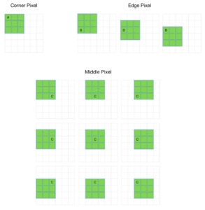
Clearly, pixel A is touched in just one convolution operation and pixel B is touched in 3 convolution operations, while pixel C is touched in 9 convolution operations. In general, pixels in the middle are used more often than pixels on corners and edges. Consequently, the information on the borders of images are not preserved as well as the information in the middle.
To overcome these problems, we use padding.
Padding Input Images
Padding is simply a process of adding layers of zeros to our input images so as to avoid the problems mentioned above.

This prevents shrinking as, if p = number of layers of zeros added to the border of the image, then our (n x n) image becomes (n + 2p) x (n + 2p) image after padding. So, applying convolution-operation (with (f x f) filter) outputs (n + 2p – f + 1) x (n + 2p – f + 1) images. For example, adding one layer of padding to an (8 x 8) image and using a (3 x 3) filter we would get an (8 x 8) output after performing convolution operation.
This increases the contribution of the pixels at the border of the original image by bringing them into the middle of the padded image. Thus, information on the borders is preserved as well as the information in the middle of the image.
Types of Padding
Valid Padding : It implies no padding at all. The input image is left in its valid/unaltered shape.
So,
[(n x n) image] * [(f x f) filter] —> [(n – f + 1) x (n – f + 1) image]
where * represents a convolution operation.
Same Padding : In this case, we add ‘p’ padding layers such that the output image has the same dimensions as the input image.
So,
[(n + 2p) x (n + 2p) image] * [(f x f) filter] —> [(n x n) image]
which gives p = (f – 1) / 2 (because n + 2p – f + 1 = n).
So, if we use a (the 3 x 3) filter the 1 layer of zeros must be added to the borders for same padding. Similarly, if (5 x 5) filter is used 2 layers of zeros must be appended to the border of the image.