")
Linear regression is a supervised learning algorithm used for computing linear relationships between input (X) and output (Y).
The steps involved in ordinary linear regression are:
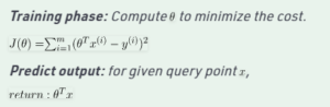

As evident from the image below, this algorithm cannot be used for making predictions when there exists a non-linear relationship between X and Y. In such cases, locally weighted linear regression is used.

Locally Weighted Linear Regression:
Locally weighted linear regression is a non-parametric algorithm, that is, the model does not learn a fixed set of parameters as is done in ordinary linear regression. Rather parameters theta are computed individually for each query point x. While computing theta, a higher “preference” is given to the points in the training set lying in the vicinity of x than the points lying far away from x.
The modified cost function is: J(theta) = $sum_{i=1}^{m} w^{(i)}(theta^Tx^{(i)} - y^{(i)})^2
where, w^{(i)} is a non-negative “weight” associated with training point x^{(i)}.
For x^{(i)}s lying closer to the query point x, the value of w^{(i)} is large, while for x^{(i)}s lying far away from x the value of w^{(i)} is small.
A typical choice of w^{(i)} is: w^{(i)} = exp(frac{-(x^{(i)} - x)^2}{2tau^2})
where, tau is called the bandwidth parameter and controls the rate at which w^{(i)} falls with distance from x
Clearly, if |x^{(i)} - x| is small w^{(i)} is close to 1 and if |x^{(i)} - x| is large w^{(i)} is close to 0.
Thus, the training-set-points lying closer to the query point x contribute more to the cost J(theta) than the points lying far away from x.
For example –
Consider a query point x = 5.0 and let x^{(1)} and x^{(2) be two points in the training set such that x^{(1)} = 4.9 and x^{(2)} = 3.0.
Using the formula w^{(i)} = exp(frac{-(x^{(i)} - x)^2}{2tau^2}) with tau = 0.5:
w^{(1)} = exp(frac{-(4.9 - 5.0)^2}{2(0.5)^2}) = 0.9802
w^{(2)} = exp(frac{-(3.0 - 5.0)^2}{2(0.5)^2}) = 0.000335
So, J(theta) = 0.9802*(theta^Tx^{(1)} - y^{(1)}) + 0.000335*(theta^Tx^{(2)} - y^{(2)})
Thus, the weights fall exponentially as the distance between x and x^{(i)} increases and so does the contribution of error in prediction for x^{(i)} to the cost.
Consequently, while computing theta, we focus more on reducing (theta^Tx^{(i)} - y^{(i)})^2 for the points lying closer to the query point (having larger value of w^{(i)}).

Steps involved in locally weighted linear regression are:
Compute theta to minimize the cost. J(theta) = $sum_{i=1}^{m} w^{(i)}(theta^Tx^{(i)} - y^{(i)})^2
Predict Output: for given query point x,
return: theta^Tx
Points to remember:
- Locally weighted linear regression is a supervised learning algorithm.
- It a non-parametric algorithm.
- There exists No training phase. All the work is done during the testing phase/while making predictions.