")
Reinforcement Learning briefly is a paradigm of Learning Process in which a learning agent learns, overtime, to behave optimally in a certain environment by interacting continuously in the environment. The agent during its course of learning experience various different situations in the environment it is in. These are called states. The agent while being in that state may choose from a set of allowable actions which may fetch different rewards(or penalties). The learning agent overtime learns to maximize these rewards so as to behave optimally at any given state it is in.
Q-Learning is a basic form of Reinforcement Learning which uses Q-values (also called action values) to iteratively improve the behavior of the learning agent.
Q-Values or Action-Values: Q-values are defined for states and actions. Q(S, A) is an estimation of how good is it to take the action A at the state S. This estimation of Q(S, A) will be iteratively computed using the TD- Update rule which we will see in the upcoming sections.
Rewards and Episodes: An agent over the course of its lifetime starts from a start state, makes a number of transitions from its current state to a next state based on its choice of action and also the environment the agent is interacting in. At every step of transition, the agent from a state takes an action, observes a reward from the environment, and then transits to another state. If at any point of time the agent ends up in one of the terminating states that means there are no further transition possible. This is said to be the completion of an episode.
Temporal Difference or TD-Update:
The Temporal Difference or TD-Update rule can be represented as follows :
This update rule to estimate the value of Q is applied at every time step of the agents interaction with the environment. The terms used are explained below. :
- S : Current State of the agent.
- A : Current Action Picked according to some policy.
- S' : Next State where the agent ends up.
- A' : Next best action to be picked using current Q-value estimation, i.e. pick the action with the maximum Q-value in the next state.
- R : Current Reward observed from the environment in Response of current action.
- $gamma$(>0 and <=1) : Discounting Factor for Future Rewards. Future rewars are less valuable than current rewards so they must be discounted. Since Q-value is an estimation of expected rewards from a state, discounting rule applies here as well.
- $alpha$ : Step length taken to update the estimation of Q(S, A).
Choosing the Action to take using $epsilon$-greedy policy:
$epsilon$-greedy policy of is a very simple policy of choosing actions using the current Q-value estimations. It goes as follows : - With probability (1-$epsilon$) choose the action which has the highest Q-value.
- With probability ($epsilon$) choose any action at random.
Now with all the theory required in hand let us take an example. We will use OpenAI’s gym environment to train our Q-Learning model.
Command to Install gym –
pip install gym
Before starting with example, you will need some helper code in order to visualize the working of the algorithms. There will be two helper files which need to be downloaded in the working directory. One can find the files here.
Step # 1 : Import required libraries.
import gym
import itertools
import matplotlib
import matplotlib.style
import numpy as np
import pandas as pd
import sys
from collections import defaultdict
from windy_gridworld import WindyGridworldEnv
import plotting
matplotlib.style.use('ggplot')
Step #2 : Create gym environment.
env = WindyGridworldEnv()
Step #3 : Make the $epsilon$-greedy policy.
def createEpsilonGreedyPolicy(Q, epsilon, num_actions):
"""
Creates an epsilon-greedy policy based
on a given Q-function and epsilon.
Returns a function that takes the state
as an input and returns the probabilities
for each action in the form of a numpy array
of length of the action space(set of possible actions).
"""
def policyFunction(state):
Action_probabilities = np.ones(num_actions,
dtype = float) * epsilon / num_actions
best_action = np.argmax(Q[state])
Action_probabilities[best_action] += (1.0 - epsilon)
return Action_probabilities
return policyFunction
Step #4 : Build Q-Learning Model.
def qLearning(env, num_episodes, discount_factor = 1.0,
alpha = 0.6, epsilon = 0.1):
"""
Q-Learning algorithm: Off-policy TD control.
Finds the optimal greedy policy while improving
following an epsilon-greedy policy"""
# Action value function
# A nested dictionary that maps
# state -> (action -> action-value).
Q = defaultdict(lambda: np.zeros(env.action_space.n))
# Keeps track of useful statistics
stats = plotting.EpisodeStats(
episode_lengths = np.zeros(num_episodes),
episode_rewards = np.zeros(num_episodes))
# Create an epsilon greedy policy function
# appropriately for environment action space
policy = createEpsilonGreedyPolicy(Q, epsilon, env.action_space.n)
# For every episode
for ith_episode in range(num_episodes):
# Reset the environment and pick the first action
state = env.reset()
for t in itertools.count():
# get probabilities of all actions from current state
action_probabilities = policy(state)
# choose action according to
# the probability distribution
action = np.random.choice(np.arange(
len(action_probabilities)),
p = action_probabilities)
# take action and get reward, transit to next state
next_state, reward, done, _ = env.step(action)
# Update statistics
stats.episode_rewards[ith_episode] += reward
stats.episode_lengths[ith_episode] = t
# TD Update
best_next_action = np.argmax(Q[next_state])
td_target = reward + discount_factor * Q[next_state][best_next_action]
td_delta = td_target - Q[state][action]
Q[state][action] += alpha * td_delta
# done is True if episode terminated
if done:
break
state = next_state
return Q, stats
Step #5 : Train the model.
Q, stats = qLearning(env, 1000)
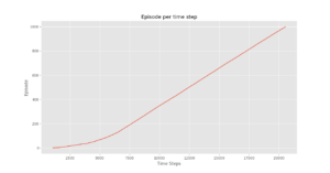
Step #6 : Plot important statistics.
plotting.plot_episode_stats(stats)

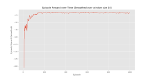
Conclusion:
We see that in the Episode Reward over time plot that the episode rewards progressively increase over time and ultimately levels out at a high reward per episode value which indicates that the agent has learnt to maximize its total reward earned in an episode by behaving optimally at every state.