")
Today, different Machine Learning techniques are used to handle different types data. One of the most difficult type of data to handle and forecast is sequential data. Sequential data is different from other types of data in the sense that while all the features of a typical dataset can be assumed to be order-independent, this cannot be assumed for a sequnetial dataset. To handle such type of data, the concept of Recurrent Neural Networks was conceived. It is different from other Artificial Neural Networks in it’s structure. While other networks “travel” in a linear direction during the feed-forward process or the back-propagation process, the Recurrent Network follows a recurrence relation instead of a feed-forward pass and uses Back-Propagation through time to learn.
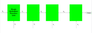
The Recurrent Neural Network consists of multiple fixed activation function units, one for each time step. Each unit has an internal state which is called the hidden state of the unit. This hidden state signifies the past knowledge that that the network currently holds at a given time step. This hidden state is updated at every time step to signify the change in the knowledge of the network about the past. The hidden state is updated using the following the recurrence relation:-
h_{t} - The new hidden state
h_{t-1} - The old hidden state
x_{t} - The current input
f_{W} - The fixed function with trainable weights
Note: Typically, to understand the concepts of a Recurrent Neural Network, it is often illustrated in it’s unrolled form and this norm will be followed in this post.
At each time step, the new hidden state is calculated using the recurrence relation as given above. This new generated hidden state is used to generate indeed a new hidden state and so on.
The basic work-flow of a Recurrent Neural Network is as follows:-
Note that h_{0} is the initial hidden state of the network. Typically, it is a vector of zeros, but it can have other values also. One method is to encode the presumptions about the data into the initial hidden state of the network. For example, for a problem to determine to the tone of a speech given by a renowned person, the person’s past speeches’ tones may be encoded into the initial hidden state. Another technique is to make the initial hidden state as a trainable parameter. Although these techniques add little nuances to the network, initializing the hidden state vector to zeros is typically an effective choice.
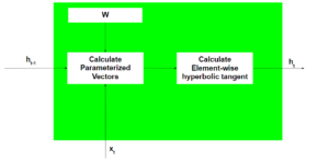
Working of each Recurrent Unit:
- Take input the previous hidden state vector and the current input vector.
Note that since the hidden state and current input are treated as vectors, each element in the vector is placed in a different dimension which is orthogonal to the other dimensions. Thus each element when multiplied by another element only gives a non-zero value when the elements involved are non-zero and the elements are in the same dimension. - Element-wise multiply the hidden state vector by the hidden state weights and similarly perform the element wise multiplication of the current input vector and the current input weights. This generates the parameterized hidden state vector and current input vector.Note that weights for different vectors are stored in the trainable weight matrix.
- Perform the vector addition of the two parameterized vectors and then calculate the element-wise hyperbolic tangent to generate the new hidden state vector.
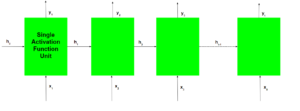
During the training of the recurrent network, the network also generates an output at each time step. This output is used to train the network using gradient descent.
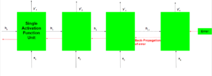
The Back-Propagation involved is similar to the one used in a typical Artificial Neural Network with some minor changes. These changes are noted as:-
Let the predicted output of the network at any time step be overline{y_{t}} and the actual output be y_{t}. Then the error at each time step is given by:-
The total error is given by the summation of the errors at all the time steps.
Similarly, the value frac{partial E}{partial W} can be calculated as the summation of gradients at each time step.
Using the chain rule of calculus and using the fact that the output at a time step t is a function of the current hidden state of the recurrent unit, the following expression arises:-
Note that the weight matrix W used in the above expression is different for the input vector and hidden state vector and is only used in this manner for notational convenience.
Thus the following expression arises:-
Thus, Back-Propagation Through Time only differs from a typical Back-Propagation in the fact the errors at each time step are summed up to calculate the total error.
Although the basic Recurrent Neural Network is fairly effective, it can suffer from a significant problem. For deep networks, The Back-Propagation process can lead to the following issues:-
Vanishing Gradients: This occurs when the gradients become very small and tend towards zero.
Exploding Gradients: This occurs when the gradients become too large due to back-propagation.
The problem of Exploding Gradients may be solved by using a hack – By putting a threshold on the gradients being passed back in time. But this solution is not seen as a solution to the problem and may also reduce the efficiency of the network. To deal with such problems, two main variants of Recurrent Neural Networks were developed – Long Short Term Memory Networks and Gated Recurrent Unit Networks.