")
Reinforcement Learning is a type of Machine Learning paradigms in which a learning algorithm is trained not on preset data but rather based on a feedback system. These algorithms are touted as the future of Machine Learning as these eliminate the cost of collecting and cleaning the data.
In this article, we are going to demonstrate how to implement a basic Reinforcement Learning algorithm which is called the Q-Learning technique. In this demonstration, we attempt to teach a bot to reach its destination using the Q-Learning technique.
Step 1: Importing the required libraries
import numpy as np
import pylab as pl
import networkx as nx
Step 2: Defining and visualising the graph
edges = [(0, 1), (1, 5), (5, 6), (5, 4), (1, 2),
(1, 3), (9, 10), (2, 4), (0, 6), (6, 7),
(8, 9), (7, 8), (1, 7), (3, 9)]
goal = 10
G = nx.Graph()
G.add_edges_from(edges)
pos = nx.spring_layout(G)
nx.draw_networkx_nodes(G, pos)
nx.draw_networkx_edges(G, pos)
nx.draw_networkx_labels(G, pos)
pl.show()

Note: The above graph may not look the same on reproduction of the code because the networkx library in python produces a random graph from the given edges.
Step 3: Defining the reward the system for the bot
MATRIX_SIZE = 11
M = np.matrix(np.ones(shape =(MATRIX_SIZE, MATRIX_SIZE)))
M *= -1
for point in edges:
print(point)
if point[1] == goal:
M[point] = 100
else:
M[point] = 0
if point[0] == goal:
M[point[::-1]] = 100
else:
M[point[::-1]]= 0
# reverse of point
M[goal, goal]= 100
print(M)
# add goal point round trip

Step 4: Defining some utility functions to be used in the training
Q = np.matrix(np.zeros([MATRIX_SIZE, MATRIX_SIZE]))
gamma = 0.75
# learning parameter
initial_state = 1
# Determines the available actions for a given state
def available_actions(state):
current_state_row = M[state, ]
available_action = np.where(current_state_row >= 0)[1]
return available_action
available_action = available_actions(initial_state)
# Chooses one of the available actions at random
def sample_next_action(available_actions_range):
next_action = int(np.random.choice(available_action, 1))
return next_action
action = sample_next_action(available_action)
def update(current_state, action, gamma):
max_index = np.where(Q[action, ] == np.max(Q[action, ]))[1]
if max_index.shape[0] > 1:
max_index = int(np.random.choice(max_index, size = 1))
else:
max_index = int(max_index)
max_value = Q[action, max_index]
Q[current_state, action] = M[current_state, action] + gamma * max_value
if (np.max(Q) > 0):
return(np.sum(Q / np.max(Q)*100))
else:
return (0)
# Updates the Q-Matrix according to the path chosen
update(initial_state, action, gamma)
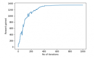
Step 5: Training and evaluating the bot using the Q-Matrix
scores = []
for i in range(1000):
current_state = np.random.randint(0, int(Q.shape[0]))
available_action = available_actions(current_state)
action = sample_next_action(available_action)
score = update(current_state, action, gamma)
scores.append(score)
# print("Trained Q matrix:")
# print(Q / np.max(Q)*100)
# You can uncomment the above two lines to view the trained Q matrix
# Testing
current_state = 0
steps = [current_state]
while current_state != 10:
next_step_index = np.where(Q[current_state, ] == np.max(Q[current_state, ]))[1]
if next_step_index.shape[0] > 1:
next_step_index = int(np.random.choice(next_step_index, size = 1))
else:
next_step_index = int(next_step_index)
steps.append(next_step_index)
current_state = next_step_index
print("Most efficient path:")
print(steps)
pl.plot(scores)
pl.xlabel('No of iterations')
pl.ylabel('Reward gained')
pl.show()
Most efficient path:
[0,1,3,9,10]
Now, Let’s bring this bot to a more realistic setting. Let us imagine that the bot is a detective and is trying to find out the location of a large drug racket. He naturally concludes that the drug sellers will not sell their products in a location which is known to be frequented by the police and the selling locations are near the location of the drug racket. Also, the sellers leave a trace of their products where they sell it and this can help the detective in finding out the required location. We want to train our bot to find the location using these Environmental Clues.
Step 6: Defining and visualizing the new graph with the environmental clues
# Defining the locations of the police and the drug traces
police = [2, 4, 5]
drug_traces = [3, 8, 9]
G = nx.Graph()
G.add_edges_from(edges)
mapping = {0:'0 - Detective', 1:'1', 2:'2 - Police', 3:'3 - Drug traces',
4:'4 - Police', 5:'5 - Police', 6:'6', 7:'7', 8:'Drug traces',
9:'9 - Drug traces', 10:'10 - Drug racket location'}
H = nx.relabel_nodes(G, mapping)
pos = nx.spring_layout(H)
nx.draw_networkx_nodes(H, pos, node_size =[200, 200, 200, 200, 200, 200, 200, 200])
nx.draw_networkx_edges(H, pos)
nx.draw_networkx_labels(H, pos)
pl.show()

Note: The above graph may look a bit different from the previous graph but they, in fact, are the same graphs. This is due to the random placement of nodes by the networkx library.
Step 7: Defining some utility functions for the training process
Q = np.matrix(np.zeros([MATRIX_SIZE, MATRIX_SIZE]))
env_police = np.matrix(np.zeros([MATRIX_SIZE, MATRIX_SIZE]))
env_drugs = np.matrix(np.zeros([MATRIX_SIZE, MATRIX_SIZE]))
initial_state = 1
# Same as above
def available_actions(state):
current_state_row = M[state, ]
av_action = np.where(current_state_row >= 0)[1]
return av_action
# Same as above
def sample_next_action(available_actions_range):
next_action = int(np.random.choice(available_action, 1))
return next_action
# Exploring the environment
def collect_environmental_data(action):
found = []
if action in police:
found.append('p')
if action in drug_traces:
found.append('d')
return (found)
available_action = available_actions(initial_state)
action = sample_next_action(available_action)
def update(current_state, action, gamma):
max_index = np.where(Q[action, ] == np.max(Q[action, ]))[1]
if max_index.shape[0] > 1:
max_index = int(np.random.choice(max_index, size = 1))
else:
max_index = int(max_index)
max_value = Q[action, max_index]
Q[current_state, action] = M[current_state, action] + gamma * max_value
environment = collect_environmental_data(action)
if 'p' in environment:
env_police[current_state, action] += 1
if 'd' in environment:
env_drugs[current_state, action] += 1
if (np.max(Q) > 0):
return(np.sum(Q / np.max(Q)*100))
else:
return (0)
# Same as above
update(initial_state, action, gamma)
def available_actions_with_env_help(state):
current_state_row = M[state, ]
av_action = np.where(current_state_row >= 0)[1]
# if there are multiple routes, dis-favor anything negative
env_pos_row = env_matrix_snap[state, av_action]
if (np.sum(env_pos_row < 0)):
# can we remove the negative directions from av_act?
temp_av_action = av_action[np.array(env_pos_row)[0]>= 0]
if len(temp_av_action) > 0:
av_action = temp_av_action
return av_action
# Determines the available actions according to the environment
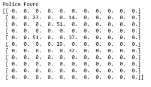
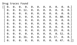
Step 8: Visualising the Environmental matrices
scores = []
for i in range(1000):
current_state = np.random.randint(0, int(Q.shape[0]))
available_action = available_actions(current_state)
action = sample_next_action(available_action)
score = update(current_state, action, gamma)
# print environmental matrices
print('Police Found')
print(env_police)
print('')
print('Drug traces Found')
print(env_drugs)
Step 9: Training and evaluating the model
scores = []
for i in range(1000):
current_state = np.random.randint(0, int(Q.shape[0]))
available_action = available_actions_with_env_help(current_state)
action = sample_next_action(available_action)
score = update(current_state, action, gamma)
scores.append(score)
pl.plot(scores)
pl.xlabel('Number of iterations')
pl.ylabel('Reward gained')
pl.show()

The example taken above was a very basic one and many practical examples like Self Driving Cars involve the concept of Game Theory.