")
Spectral Clustering is a growing clustering algorithm which has performed better than many traditional clustering algorithms in many cases. It treats each data point as a graph-node and thus transforms the clustering problem into a graph-partitioning problem. A typical implementation consists of three fundamental steps:-
- Building the Similarity Graph: This step builds the Similarity Graph in the form of an adjacency matrix which is represented by A. The adjacency matrix can be built in the following manners:-
- Epsilon-neighbourhood Graph: A parameter epsilon is fixed beforehand. Then, each point is connected to all the points which lie in it’s epsilon-radius. If all the distances between any two points are similar in scale then typically the weights of the edges ie the distance between the two points are not stored since they do not provide any additional information. Thus, in this case, the graph built is an undirected and unweighted graph.
- K-Nearest Neighbours A parameter k is fixed beforehand. Then, for two vertices u and v, an edge is directed from u to v only if v is among the k-nearest neighbours of u. Note that this leads to the formation of a weighted and directed graph because it is not always the case that for each u having v as one of the k-nearest neighbours, it will be the same case for v having u among its k-nearest neighbours. To make this graph undirected, one of the following approaches are followed:-
1. Direct an edge from u to v and from v to u if either v is among the k-nearest neighbours of u OR u is among the k-nearest neighbours of v.
2. Direct an edge from u to v and from v to u if v is among the k-nearest neighbours of u AND u is among the k-nearest neighbours of v. - Fully-Connected Graph: To build this graph, each point is connected with an undirected edge-weighted by the distance between the two points to every other point. Since this approach is used to model the local neighbourhood relationships thus typically the Gaussian similarity metric is used to calculate the distance.
2. Projecting the data onto a lower Dimensional Space: This step is done to account for the possibility that members of the same cluster may be far away in the given dimensional space. Thus the dimensional space is reduced so that those points are closer in the reduced dimensional space and thus can be clustered together by a traditional clustering algorithm. It is done by computing the Graph Laplacian Matrix . To compute it though first, the degree of a node needs to be defined. The degree of the ith node is given by
Note that w_{ij} is the edge between the nodes i and j as defined in the adjacency matrix above.
The degree matrix is defined as follows:-
Thus the Graph Laplacian Matrix is defined as:-
L = D-A
This Matrix is then normalized for mathematical efficiency. To reduce the dimensions, first, the eigenvalues and the respective eigenvectors are calculated. If the number of clusters is k then the first eigenvalues and their eigen-vectors are taken and stacked into a matrix such that the eigen-vectors are the columns.
3. Clustering the Data: This process mainly involves clustering the reduced data by using any traditional clustering technique – typically K-Means Clustering. First, each node is assigned a row of the normalized of the Graph Laplacian Matrix. Then this data is clustered using any traditional technique. To transform the clustering result, the node identifier is retained.
Properties:
4. Assumption-Less: This clustering technique, unlike other traditional techniques do not assume the data to follow some property. Thus this makes this technique to answer a more-generic class of clustering problems.
Ease of implementation and Speed: This algorithm is easier to implement than other clustering algorithms and is also very fast as it mainly consists of mathematical computations.
Not-Scalable: Since it involves the building of matrices and computation of eigenvalues and eigenvectors it is time-consuming for dense datasets.
The below steps demonstrate how to implement Spectral Clustering using Sklearn. The data for the following steps is the Credit Card Data which can be downloaded from Kaggle.
Step 1: Importing the required libraries
import pandas as pd
import matplotlib.pyplot as plt
from sklearn.cluster import SpectralClustering
from sklearn.preprocessing import StandardScaler, normalize
from sklearn.decomposition import PCA
from sklearn.metrics import silhouette_score
Step 2: Loading and Cleaning the Data
# Changing the working location to the location of the data
cd "C:UsersDevDesktopKaggleCredit_Card"
# Loading the data
X = pd.read_csv('CC_GENERAL.csv')
# Dropping the CUST_ID column from the data
X = X.drop('CUST_ID', axis = 1)
# Handling the missing values if any
X.fillna(method ='ffill', inplace = True)
X.head()
Step 3: Preprocessing the data to make the data visualizable
# Preprocessing the data to make it visualizable
# Scaling the Data
scaler = StandardScaler()
X_scaled = scaler.fit_transform(X)
# Normalizing the Data
X_normalized = normalize(X_scaled)
# Converting the numpy array into a pandas DataFrame
X_normalized = pd.DataFrame(X_normalized)
# Reducing the dimensions of the data
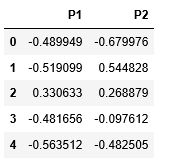
pca = PCA(n_components = 2)
X_principal = pca.fit_transform(X_normalized)
X_principal = pd.DataFrame(X_principal)
X_principal.columns = ['P1', 'P2']
X_principal.head()
Step 4: Building the Clustering models and Visualizing the clustering
In the below steps, two different Spectral Clustering models with different values for the parameter ‘affinity’. You can read about the documentation of the Spectral Clustering class here.
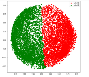
a) affinity = ‘rbf’
# Building the clustering model
spectral_model_rbf = SpectralClustering(n_clusters = 2, affinity ='rbf')
# Training the model and Storing the predicted cluster labels
labels_rbf = spectral_model_rbf.fit_predict(X_principal)
# Building the label to colour mapping
colours = {}
colours[0] = 'b'
colours[1] = 'y'
# Building the colour vector for each data point
cvec = [colours[label] for label in labels_rbf]
# Plotting the clustered scatter plot
b = plt.scatter(X_principal['P1'], X_principal['P2'], color ='b');
y = plt.scatter(X_principal['P1'], X_principal['P2'], color ='y');
plt.figure(figsize =(9, 9))
plt.scatter(X_principal['P1'], X_principal['P2'], c = cvec)
plt.legend((b, y), ('Label 0', 'Label 1'))
plt.show()

b) affinity = ‘nearest_neighbors’
# Building the clustering model
spectral_model_nn = SpectralClustering(n_clusters = 2, affinity ='nearest_neighbors')
# Training the model and Storing the predicted cluster labels
labels_nn = spectral_model_nn.fit_predict(X_principal)
Step 5: Evaluating the performances
# List of different values of affinity
affinity = ['rbf', 'nearest-neighbours']
# List of Silhouette Scores
s_scores = []
# Evaluating the performance
s_scores.append(silhouette_score(X, labels_rbf))
s_scores.append(silhouette_score(X, labels_nn))
print(s_scores)
![]()
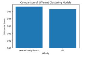
Step 6: Comparing the performances
# Plotting a Bar Graph to compare the models
plt.bar(affinity, s_scores)
plt.xlabel('Affinity')
plt.ylabel('Silhouette Score')
plt.title('Comparison of different Clustering Models')
plt.show()