")
When Regression is chosen?
A regression problem is when the output variable is a real or continuous value, such as “salary” or “weight”. Many different models can be used, the simplest is the linear regression. It tries to fit data with the best hyperplane which goes through the points.
Regression Analysis is a statistical process for estimating the relationships between the dependent variables or criterion variables and one or more independent variables or predictors. Regression analysis explains the changes in criterions in relation to changes in select predictors. The conditional expectation of the criterions based on predictors where the average value of the dependent variables is given when the independent variables are changed. Three major uses for regression analysis are determining the strength of predictors, forecasting an effect, and trend forecasting.
Types of Regression –
- Linear regression
- Logistic regression
- Polynomial regression
- Stepwise regression
- Stepwise regression
- Ridge regression
- Lasso regression
- ElasticNet regression
Linear regression is used for predictive analysis. Linear regression is a linear approach for modeling the relationship between the criterion or the scalar response and the multiple predictors or explanatory variables. Linear regression focuses on the conditional probability distribution of the response given the values of the predictors. For linear regression, there is a danger of overfitting. The formula for linear regression is: Y’ = bX + A.
Logistic regression is used when the dependent variable is dichotomous. Logistic regression estimates the parameters of a logistic model and is form of binomial regression. Logistic regression is used to deal with data that has two possible criterions and the relationship between the criterions and the predictors. The equation for logistic regression is: l = beta_{0}+beta_{1}x_{1}+beta_{2}x_{2}.
Polynomial regression is used for curvilinear data. Polynomial regression is fit with the method of least squares. The goal of regression analysis to model the expected value of a dependent variable y in regards to the independent variable x. The equation for polynomial regression is: l = beta_{0}+beta_{0}x_{1}+epsilon.
Stepwise regression is used for fitting regression models with predictive models. It is carried out automatically. With each step, the variable is added or subtracted from the set of explanatory variables. The approaches for stepwise regression are forward selection, backward elimination, and bidirectional elimination. The formula for stepwise regression is b_{j.std} = b_{j}(s_{x} * s_{y}^{-1}).
Ridge regression is a technique for analyzing multiple regression data. When multicollinearity occurs, least squares estimates are unbiased. A degree of bias is added to the regression estimates, and a result, ridge regression reduces the standard errors. The formula for ridge regression is beta = (X^{T}X + lambda * I)^{-1}X^{T}y.
Lasso regression is a regression analysis method that performs both variable selection and regularization. Lasso regression uses soft thresholding. Lasso regression selects only a subset of the provided covariates for use in the final model. Lasso regression is N^{-1}sum^{N}_{i=1}f(x_{i}, y_{I}, alpha, beta).
ElasticNet regression is a regularized regression method that linearly combines the penalties of the lasso and ridge methods. ElasticNet regression is used for support vector machines, metric learning, and portfolio optimization. The penalty function is given by:||beta||_{1} = sum^{p}_{j=1}|beta_{j}|.
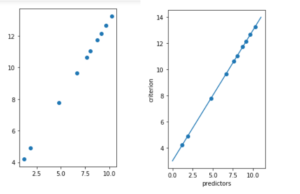
Below is the simple implementation:
# importing libraries
import numpy as np
import matplotlib.pyplot as plt
from sklearn.linear_model import LinearRegression
x = 11 * np.random.random((10, 1))
# y = a * x + b
y = 1.0 * x + 3.0
# create a linear regression model
model = LinearRegression()
model.fit(x, y)
# predict y from the data where the x is predicted from the x
X_prediction = np.linspace(0, 11, 100)
Y_prediction = model.predict(X_prediction[:, np.newaxis])
# plot the results
plt.figure(figsize =(3, 5))
co_X = plt.axes()
co_X.scatter(x, y)
co_X.plot(X_prediction, Y_prediction)
co_X.set_xlabel('predictors')
co_X.set_ylabel('criterion')
co_X.axis('tight')
plt.show()
Output: