")
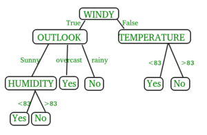
Decision Tree is one of the most powerful and popular algorithm. Decision-tree algorithm falls under the category of supervised learning algorithms. It works for both continuous as well as categorical output variables.

In this article, We are going to implement a Decision tree algorithm on the Balance Scale Weight & Distance Database presented on the UCI.
Data-set Description :
Title : Balance Scale Weight & Distance Database
Number of Instances: 625 (49 balanced, 288 left, 288 right)
Number of Attributes: 4 (numeric) + class name = 5
Attribute Information:
Class Name (Target variable): 3
L [balance scale tip to the left]
B [balance scale be balanced]
R [balance scale tip to the right]
Left-Weight: 5 (1, 2, 3, 4, 5)
Left-Distance: 5 (1, 2, 3, 4, 5)
Right-Weight: 5 (1, 2, 3, 4, 5)
Right-Distance: 5 (1, 2, 3, 4, 5)
Missing Attribute Values: None
Class Distribution:
46.08 percent are L
07.84 percent are B
46.08 percent are R
You can find more details of the dataset here.
Used Python Packages :
sklearn :
In python, sklearn is a machine learning package which include a lot of ML algorithms.
Here, we are using some of its modules like train_test_split, DecisionTreeClassifier and accuracy_score.
NumPy :
It is a numeric python module which provides fast maths functions for calculations.
It is used to read data in numpy arrays and for manipulation purpose.
Pandas :
Used to read and write different files.
Data manipulation can be done easily with dataframes.
Installation of the packages :
In Python, sklearn is the package which contains all the required packages to implement Machine learning algorithm. You can install the sklearn package by following the commands given below.
using pip :
pip install -U scikit-learn
Before using the above command make sure you have scipy and numpy packages installed.
If you don’t have pip. You can install it using
python get-pip.py
using conda :
conda install scikit-learn
Assumptions we make while using Decision tree :
At the beginning, we consider the whole training set as the root.
Attributes are assumed to be categorical for information gain and for gini index, attributes are assumed to be continuous.
On the basis of attribute values records are distributed recursively.
We use statistical methods for ordering attributes as root or internal node.
Pseudocode :
Find the best attribute and place it on the root node of the tree.
Now, split the training set of the dataset into subsets. While making the subset make sure that each subset of training dataset should have the same value for an attribute.
Find leaf nodes in all branches by repeating 1 and 2 on each subset.
While implementing the decision tree we will go through the following two phases:
- Building Phase
- Preprocess the dataset.
- Split the dataset from train and test using Python sklearn package.
- Train the classifier.
2. Operational Phase
- Make predictions.
- Calculate the accuracy.
Data Import :
- To import and manipulate the data we are using the pandas package provided in python.
- Here, we are using a URL which is directly fetching the dataset from the UCI site no need to download the dataset. When you try to run this code on your system make sure the system should have an active Internet connection.
- As the dataset is separated by “,” so we have to pass the sep parameter’s value as “,”.
Another thing is notice is that the dataset doesn’t contain the header so we will pass the Header parameter’s value as none. If we will not pass the header parameter then it will consider the first line of the dataset as the header.
Data Slicing :
- Before training the model we have to split the dataset into the training and testing dataset.
- To split the dataset for training and testing we are using the sklearn module train_test_split
- First of all we have to separate the target variable from the attributes in the dataset.
X = balance_data.values[:, 1:5]
Y = balance_data.values[:,0] - Above are the lines from the code which separate the dataset. The variable X contains the attributes while the variable Y contains the target variable of the dataset.
- Next step is to split the dataset for training and testing purpose.
x-train, X-test, y-train, y-test = train_test_split(
X, Y, test-size = 0.3, random-state = 100) - Above line split the dataset for training and testing. As we are splitting the dataset in a ratio of 70:30 between training and testing so we are pass test-size parameter’s value as 0.3.
random-state variable is a pseudo-random number generator state used for random sampling.
Terms used in code :
Gini index and information gain both of these methods are used to select from the n attributes of the dataset which attribute would be placed at the root node or the internal node.
Gini index
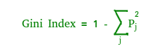
- Gini Index is a metric to measure how often a randomly chosen element would be incorrectly identified.
- It means an attribute with lower gini index should be preferred.
- Sklearn supports “gini” criteria for Gini Index and by default, it takes “gini” value.
Entropy
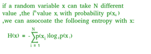
- Entropy is the measure of uncertainty of a random variable, it characterizes the impurity of an arbitrary collection of examples. The higher the entropy the more the information content.
Information Gain
- The entropy typically changes when we use a node in a decision tree to partition the training instances into smaller subsets. Information gain is a measure of this change in entropy.
- Sklearn supports “entropy” criteria for Information Gain and if we want to use Information Gain method in sklearn then we have to mention it explicitly.
Accuracy score - Accuracy score is used to calculate the accuracy of the trained classifier.
Confusion Matrix - Confusion Matrix is used to understand the trained classifier behavior over the test dataset or validate dataset.
Recommended: Please try your approach on {IDE} first, before moving on to the solution.
Below is the python code for the decision tree.
# Run this program on your local python
# interpreter, provided you have installed
# the required libraries.
# Importing the required packages
import numpy as np
import pandas as pd
from sklearn.metrics import confusion_matrix
from sklearn.cross_validation import train_test_split
from sklearn.tree import DecisionTreeClassifier
from sklearn.metrics import accuracy_score
from sklearn.metrics import classification_report
# Function importing Dataset
def importdata():
balance_data = pd.read_csv(
'https://archive.ics.uci.edu/ml/machine-learning-'+
'databases/balance-scale/balance-scale.data',
sep= ',', header = None)
# Printing the dataswet shape
print ("Dataset Length: ", len(balance_data))
print ("Dataset Shape: ", balance_data.shape)
# Printing the dataset obseravtions
print ("Dataset: ",balance_data.head())
return balance_data
# Function to split the dataset
def splitdataset(balance_data):
# Separating the target variable
X = balance_data.values[:, 1:5]
Y = balance_data.values[:, 0]
# Splitting the dataset into train and test
x-train, X-test, y-train, y-test = train_test_split(
X, Y, test-size = 0.3, random-state = 100)
return X, Y, x-train, X-test, y-train, y-test
# Function to perform training with giniIndex.
def train_using_gini(x-train, X-test, y-train):
# Creating the classifier object
clf_gini = DecisionTreeClassifier(criterion = "gini",
random-state = 100,max_depth=3, min_samples_leaf=5)
# Performing training
clf_gini.fit(x-train, y-train)
return clf_gini
# Function to perform training with entropy.
def tarin_using_entropy(x-train, X-test, y-train):
# Decision tree with entropy
clf_entropy = DecisionTreeClassifier(
criterion = "entropy", random-state = 100,
max_depth = 3, min_samples_leaf = 5)
# Performing training
clf_entropy.fit(x-train, y-train)
return clf_entropy
# Function to make predictions
def prediction(X-test, clf_object):
# Predicton on test with giniIndex
Y_prediction = clf_object.predict(X-test)
print("Predicted values:")
print(Y_prediction)
return Y_prediction
# Function to calculate accuracy
def cal_accuracy(y-test, Y_prediction):
print("Confusion Matrix: ",
confusion_matrix(y-test, Y_prediction))
print ("Accuracy : ",
accuracy_score(y-test,Y_prediction)*100)
print("Report : ",
classification_report(y-test, Y_prediction))
# Driver code
def main():
# Building Phase
data = importdata()
X, Y, x-train, X-test, y-train, y-test = splitdataset(data)
clf_gini = train_using_gini(x-train, X-test, y-train)
clf_entropy = tarin_using_entropy(x-train, X-test, y-train)
# Operational Phase
print("Results Using Gini Index:")
# Prediction using gini
Y_prediction_gini = prediction(X-test, clf_gini)
cal_accuracy(y-test, Y_prediction_gini)
print("Results Using Entropy:")
# Prediction using entropy
Y_prediction_entropy = prediction(X-test, clf_entropy)
cal_accuracy(y-test, Y_prediction_entropy)
# Calling main function
if __name__=="__main__":
main()
Data Infomation:
Dataset Length: 625
Dataset Shape: (625, 5)
Dataset: 0 1 2 3 4
0 B 1 1 1 1
1 R 1 1 1 2
2 R 1 1 1 3
3 R 1 1 1 4
4 R 1 1 1 5
Results Using Gini Index:
Predicted values:
['R' 'L' 'R' 'R' 'R' 'L' 'R' 'L' 'L' 'L' 'R' 'L' 'L' 'L' 'R' 'L' 'R' 'L'
'L' 'R' 'L' 'R' 'L' 'L' 'R' 'L' 'L' 'L' 'R' 'L' 'L' 'L' 'R' 'L' 'L' 'L'
'L' 'R' 'L' 'L' 'R' 'L' 'R' 'L' 'R' 'R' 'L' 'L' 'R' 'L' 'R' 'R' 'L' 'R'
'R' 'L' 'R' 'R' 'L' 'L' 'R' 'R' 'L' 'L' 'L' 'L' 'L' 'R' 'R' 'L' 'L' 'R'
'R' 'L' 'R' 'L' 'R' 'R' 'R' 'L' 'R' 'L' 'L' 'L' 'L' 'R' 'R' 'L' 'R' 'L'
'R' 'R' 'L' 'L' 'L' 'R' 'R' 'L' 'L' 'L' 'R' 'L' 'R' 'R' 'R' 'R' 'R' 'R'
'R' 'L' 'R' 'L' 'R' 'R' 'L' 'R' 'R' 'R' 'R' 'R' 'L' 'R' 'L' 'L' 'L' 'L'
'L' 'L' 'L' 'R' 'R' 'R' 'R' 'L' 'R' 'R' 'R' 'L' 'L' 'R' 'L' 'R' 'L' 'R'
'L' 'L' 'R' 'L' 'L' 'R' 'L' 'R' 'L' 'R' 'R' 'R' 'L' 'R' 'R' 'R' 'R' 'R'
'L' 'L' 'R' 'R' 'R' 'R' 'L' 'R' 'R' 'R' 'L' 'R' 'L' 'L' 'L' 'L' 'R' 'R'
'L' 'R' 'R' 'L' 'L' 'R' 'R' 'R']
Confusion Matrix: [[ 0 6 7]
[ 0 67 18]
[ 0 19 71]]
Accuracy : 73.4042553191
Report :
precision recall f1-score support
B 0.00 0.00 0.00 13
L 0.73 0.79 0.76 85
R 0.74 0.79 0.76 90
avg/total 0.68 0.73 0.71 188
Results Using Entropy:
Predicted values:
['R' 'L' 'R' 'L' 'R' 'L' 'R' 'L' 'R' 'R' 'R' 'R' 'L' 'L' 'R' 'L' 'R' 'L'
'L' 'R' 'L' 'R' 'L' 'L' 'R' 'L' 'R' 'L' 'R' 'L' 'R' 'L' 'R' 'L' 'L' 'L'
'L' 'L' 'R' 'L' 'R' 'L' 'R' 'L' 'R' 'R' 'L' 'L' 'R' 'L' 'L' 'R' 'L' 'L'
'R' 'L' 'R' 'R' 'L' 'R' 'R' 'R' 'L' 'L' 'R' 'L' 'L' 'R' 'L' 'L' 'L' 'R'
'R' 'L' 'R' 'L' 'R' 'R' 'R' 'L' 'R' 'L' 'L' 'L' 'L' 'R' 'R' 'L' 'R' 'L'
'R' 'R' 'L' 'L' 'L' 'R' 'R' 'L' 'L' 'L' 'R' 'L' 'L' 'R' 'R' 'R' 'R' 'R'
'R' 'L' 'R' 'L' 'R' 'R' 'L' 'R' 'R' 'L' 'R' 'R' 'L' 'R' 'R' 'R' 'L' 'L'
'L' 'L' 'L' 'R' 'R' 'R' 'R' 'L' 'R' 'R' 'R' 'L' 'L' 'R' 'L' 'R' 'L' 'R'
'L' 'R' 'R' 'L' 'L' 'R' 'L' 'R' 'R' 'R' 'R' 'R' 'L' 'R' 'R' 'R' 'R' 'R'
'R' 'L' 'R' 'L' 'R' 'R' 'L' 'R' 'L' 'R' 'L' 'R' 'L' 'L' 'L' 'L' 'L' 'R'
'R' 'R' 'L' 'L' 'L' 'R' 'R' 'R']
Confusion Matrix: [[ 0 6 7]
[ 0 63 22]
[ 0 20 70]]
Accuracy : 70.7446808511
Report :
precision recall f1-score support
B 0.00 0.00 0.00 13
L 0.71 0.74 0.72 85
R 0.71 0.78 0.74 90
avg / total 0.66 0.71 0.68 188