")
- Decision tree algorithm falls under the category of supervised learning. They can be used to solve both regression and classification problems.
- Decision tree uses the tree representation to solve the problem in which each leaf node corresponds to a class label and attributes are represented on the internal node of the tree.
- We can represent any boolean function on discrete attributes using the decision tree.

Below are some assumptions that we made while using decision tree:
- At the beginning, we consider the whole training set as the root.
- Feature values are preferred to be categorical. If the values are continuous then they are discretized prior to building the model.
- On the basis of attribute values records are distributed recursively.
- We use statistical methods for ordering attributes as root or the internal node.
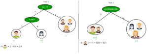
As you can see from the above image that Decision Tree works on the Sum of Product form which is also known as Disjunctive Normal Form. In the above image, we are predicting the use of computer in the daily life of the people.
In Decision Tree the major challenge is to identification of the attribute for the root node in each level. This process is known as attribute selection. We have two popular attribute selection measures:
Information Gain
Gini Index
1. Information Gain
When we use a node in a decision tree to partition the training instances into smaller subsets the entropy changes. Information gain is a measure of this change in entropy.
Definition: Suppose S is a set of instances, A is an attribute, Sv is the subset of S with A = v, and Values (A) is the set of all possible values of A, then
Gain(S, A) = Entropy(S) - sum_{v epsilon Values(A)}frac{left | S_{v} right |}{left | S right |}. Entropy(S_{v})
Entropy
Entropy is the measure of uncertainty of a random variable, it characterizes the impurity of an arbitrary collection of examples. The higher the entropy more the information content.
Definition: Suppose S is a set of instances, A is an attribute, Sv is the subset of S with A = v, and Values (A) is the set of all possible values of A, then
Gain(S, A) = Entropy(S) - sum_{v epsilon Values(A)}frac{left | S_{v} right |}{left | S right |}. Entropy(S_{v})
Example:
For the set X = {a,a,a,b,b,b,b,b}
Total intances: 8
Instances of b: 5
Instances of a: 3
Entropy H(X) = -left [ left ( frac{3}{8} right )log_{2}frac{3}{8} + left ( frac{5}{8} right )log_{2}frac{5}{8} right ]
= -[0.375 * (-1.415) + 0.625 * (-0.678)]
=-(-0.53-0.424)
= 0.954
Building Decision Tree using Information Gain
The essentials:
- Start with all training instances associated with the root node
- Use info gain to choose which attribute to label each node with
- Note: No root-to-leaf path should contain the same discrete attribute twice
- Recursively construct each subtree on the subset of training instances that would be classified down that path in the tree.
The border cases:
- If all positive or all negative training instances remain, label that node “yes” or “no” accordingly
- If no attributes remain, label with a majority vote of training instances left at that node
- If no instances remain, label with a majority vote of the parent’s training instances
Example:
Now, lets draw a Decision Tree for the following data using Information gain.
Training set: 3 features and 2 classes
X Y Z C
1 1 1 I
1 1 0 I
0 0 1 II
1 0 0 II
Here, we have 3 features and 2 output classes.
To build a decision tree using Information gain. We will take each of the feature and calculate the information for each feature.
Split on feature X

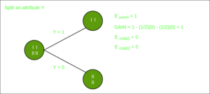
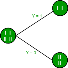
Split on feature Y
Split on feature Z

From the above images we can see that the information gain is maximum when we make a split on feature Y. So, for the root node best suited feature is feature Y. Now we can see that while splitting the dataset by feature Y, the child contains pure subset of the target variable. So we don’t need to further split the dataset.
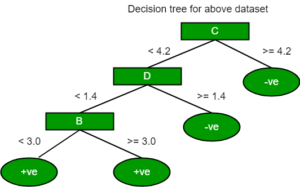
The final tree for the above dataset would be look like this:
2. Gini Index
Gini Index is a metric to measure how often a randomly chosen element would be incorrectly identified.
It means an attribute with lower Gini index should be preferred.
Sklearn supports “Gini” criteria for Gini Index and by default, it takes “gini” value.
The Formula for the calculation of the of the Gini Index is given below.
Gini Index = 1 - sum_{j}^{}p_{j}^{2}
Example:
Lets consider the dataset in the image below and draw a decision tree using gini index.
Index A B C D E
1 4.8 3.4 1.9 0.2 positive
2 5 3 1.6 1.2 positive
3 5 3.4 1.6 0.2 positive
4 5.2 3.5 1.5 0.2 positive
5 5.2 3.4 1.4 0.2 positive
6 4.7 3.2 1.6 0.2 positive
7 4.8 3.1 1.6 0.2 positive
8 5.4 3.4 1.5 0.4 positive
9 7 3.2 4.7 1.4 negative
10 6.4 3.2 4.7 1.5 negative
11 6.9 3.1 4.9 1.5 negative
12 5.5 2.3 4 1.3 negative
13 6.5 2.8 4.6 1.5 negative
14 5.7 2.8 4.5 1.3 negative
15 6.3 3.3 4.7 1.6 negative
16 4.9 2.4 3.3 1 negative
In the dataset above there are 5 attributes from which attribute E is the predicting feature which contains 2(Positive & Negative) classes. We have an equal proportion for both the classes.
In Gini Index, we have to choose some random values to categorize each attribute. These values for this dataset are:
A B C D
>= 5 >= 3.0 >= 4.2 >= 1.4
< 5 < 3.0 < 4.2 < 1.4
Calculating Gini Index for Var A:
Value >= 5: 12
Attribute A >= 5 & class = positive: frac{5}{12}
Attribute A >= 5 & class = negative: frac{7}{12}
Gini(5, 7) = 1 – left [ left ( frac{5}{12} right )^{2} + left ( frac{7}{12} right )^{2}right ] = 0.4860
Value < 5: 4
Attribute A < 5 & class = positive: frac{3}{4}
Attribute A < 5 & class = negative: frac{1}{4}
Gini(3, 1) = 1 – left [ left ( frac{3}{4} right )^{2} + left ( frac{1}{4} right )^{2}right ] = 0.375
By adding weight and sum each of the gini indices:
gini(Target, A) = left ( frac{12}{16} right ) * (0.486) + left ( frac{4}{16} right ) * (0.375) = 0.45825
Calculating Gini Index for Var B:
Value >= 3: 12
Attribute B >= 3 & class = positive: frac{8}{12}
Attribute B >= 5 & class = negative: frac{4}{12}
Gini(5, 7) = 1 – left [ left ( frac{8}{12} right )^{2} + left ( frac{4}{12} right )^{2}right ] = 0.4460
Value < 3: 4
Attribute A < 3 & class = positive: frac{0}{4}
Attribute A < 3 & class = negative: frac{4}{4}
Gini(3, 1) = 1 – left [ left ( frac{0}{4} right )^{2} + left ( frac{4}{4} right )^{2}right ] = 1
By adding weight and sum each of the gini indices:
gini(Target, B) = left ( frac{12}{16} right ) * (0.446) + left ( frac{0}{16} right ) * (0) = 0.3345
Using the same approach we can calculate the Gini index for C and D attributes.
Positive Negative
For A|>= 5.0 5 7
|<5 3 1
Ginin Index of A = 0.45825
Positive Negative
For B|>= 3.0 8 4
|< 3.0 0 4
Gini Index of B= 0.3345
Positive Negative
For C|>= 4.2 0 6
|< 4.2 8 2
Gini Index of C= 0.2
Positive Negative
For D|>= 1.4 0 5
|< 1.4 8 3
Gini Index of D= 0.273
The most notable types of decision tree algorithms are:-
1. Iterative Dichotomiser 3 (ID3): This algorithm uses Information Gain to decide which attribute is to be used classify the current subset of the data. For each level of the tree, information gain is calculated for the remaining data recursively.
2. C4.5: This algorithm is the successor of the ID3 algorithm. This algorithm uses either Information gain or Gain ratio to decide upon the classifying attribute. It is a direct improvement from the ID3 algorithm as it can handle both continuous and missing attribute values.
3. Classification and Regression Tree(CART): It is a dynamic learning algorithm which can produce a regression tree as well as a classification tree depending upon the dependent variable.