")
Decision Tree is a decision-making tool that uses a flowchart-like tree structure or is a model of decisions and all of their possible results, including outcomes, input costs and utility.
Decision-tree algorithm falls under the category of supervised learning algorithms. It works for both continuous as well as categorical output variables.
The branches/edges represent the result of the node and the nodes have either:
Conditions [Decision Nodes]
Result [End Nodes]
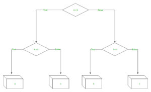
The branches/edges represent the truth/falsity of the statement and takes makes a decision based on that in the example below which shows a decision tree that evaluates the smallest of three numbers:
Decision Tree Regression:
Decision tree regression observes features of an object and trains a model in the structure of a tree to predict data in the future to produce meaningful continuous output. Continuous output means that the output/result is not discrete, i.e., it is not represented just by a discrete, known set of numbers or values.
Discrete output example: A weather prediction model that predicts whether or not there’ll be rain in a particular day.
Continuous output example: A profit prediction model that states the probable profit that can be generated from the sale of a product.
Here, continuous values are predicted with the help of a decision tree regression model.
Let’s see the Step-by-Step implementation –
Step 1: Import the required libraries.
# import numpy package for arrays and stuff
import numpy as np
# import matplotlib.pyplot for plotting our result
import matplotlib.pyplot as plt
# import pandas for importing csv files
import pandas as pd
Step 2: Initialize and print the Dataset.
# import dataset
# dataset = pd.read_csv('Data.csv')
# alternatively open up .csv file to read data
dataset = np.array(
[['Asset Flip', 100, 1000],
['Text Based', 500, 3000],
['Visual Novel', 1500, 5000],
['2D Pixel Art', 3500, 8000],
['2D Vector Art', 5000, 6500],
['Strategy', 6000, 7000],
['First Person Shooter', 8000, 15000],
['Simulator', 9500, 20000],
['Racing', 12000, 21000],
['RPG', 14000, 25000],
['Sandbox', 15500, 27000],
['Open-World', 16500, 30000],
['MMOFPS', 25000, 52000],
['MMORPG', 30000, 80000]
])
# print the dataset
print(dataset)

Step 3: Select all the rows and column 1 from dataset to “X”.
# select all rows by : and column 1
# by 1:2 representing features
X = dataset[:, 1:2].astype(int)
# print X
print(X)

Step 4: Select all of the rows and column 2 from dataset to “y”.
# select all rows by : and column 2
# by 2 to Y representing labels
y = dataset[:, 2].astype(int)
# print y
print(y)
![]()
Step 5: Fit decision tree regressor to the dataset
# import the regressor
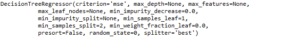
from sklearn.tree import DecisionTreeRegressor
# create a regressor object
regressor = DecisionTreeRegressor(random-state = 0)
# fit the regressor with X and Y data
regressor.fit(X, y)
Step 6: Predicting a new value
# predicting a new value
# test the output by changing values, like 3750
Y_prediction = regressor.predict(3750)
# print the predicted price
print("Predicted price: % dn"% Y_prediction)
Predicted Price : 8000
Step 7: Visualising the result
# arange for creating a range of values
# from min value of X to max value of X
# with a difference of 0.01 between two
# consecutive values
X_grid = np.arange(min(X), max(X), 0.01)
# reshape for reshaping the data into
# a len(X_grid)*1 array, i.e. to make
# a column out of the X_grid values
X_grid = X_grid.reshape((len(X_grid), 1))
# scatter plot for original data
plt.scatter(X, y, color = 'red')
# plot predicted data
plt.plot(X_grid, regressor.predict(X_grid), color = 'blue')
# specify title
plt.title('Profit to Production Cost (Decision Tree Regression)')
# specify X axis label
plt.xlabel('Production Cost')
# specify Y axis label
plt.ylabel('Profit')
# show the plot
plt.show()

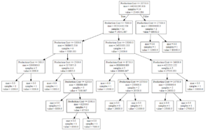
Step 8: The tree is finally exported and shown in the TREE STRUCTURE below, visualized using http://www.webgraphviz.com/ by copying the data from the ‘tree.dot’ file.
# import export_graphviz
from sklearn.tree import export_graphviz
# export the decision tree to a tree.dot file
# for visualizing the plot easily anywhere
export_graphviz(regressor, out_file ='tree.dot',
feature_names =['Production Cost'])
Output (Decision Tree):