")
Linear Regression :
It is a commonly used type of predictive analysis. It is a statistical approach for modelling relationship between a dependent variable and a given set of independent variables.
There are two types of linear regression.
- Simple Linear Regression
- Multiple Linear Regression
Let’s discuss Simple Linear regression using R.
Simple Linear Regression:
It is a statistical method that allows us to summarize and study relationships between two continuous (quantitative) variables. One variable denoted x is regarded as an independent variable and other one denoted y is regarded as a dependent variable. It is assumed that the two variables are linearly related. Hence, we try to find a linear function that predicts the response value(y) as accurately as possible as a function of the feature or independent variable(x).
For understanding the concept let’s consider a salary dataset where it is given the value of the dependent variable(salary) for every independent variable(years experienced).
Salary dataset-
Years experienced Salary
1.1 39343.00
1.3 46205.00
1.5 37731.00
2.0 43525.00
2.2 39891.00
2.9 56642.00
3.0 60150.00
3.2 54445.00
3.2 64445.00
3.7 57189.00
For general purpose, we define:
x as a feature vector, i.e x = [x_1, x_2, …., x_n],
y as a response vector, i.e y = [y_1, y_2, …., y_n]
for n observations (in above example, n=10).
Scatter plot of given dataset:

Now, we have to find a line which fits the above scatter plot through which we can predict any value of y or response for any value of x
The lines which best fits is called Regression line.
The equation of regression line is given by:
y = a + bx
Where y is predicted response value, a is y intercept, x is feature value and b is slope.
To create the model, let’s evaluate the values of regression coefficient a and b. And as soon as the estimation of these coefficients is done, the response model can be predicted. Here we are going to use Least Square Technique.
The principle of least squares is one of the popular methods for finding a curve fitting a given data. Say (x1, y1), (x2, y2)….(xn, yn) be n observations from an experiment. We are interested in finding a curve
y=f(x) .....(1)
Closely fitting the given data of size ‘n’. Now at x=x1 while the observed value of y is y1 the expected value of y from curve (1) is f(x1).Then the residual can be defined by…
e1=y1-f(x1) ...(2)
Similarly residual for x2, x3…xn are given by …
e2=y2-f(x2) .....(3)
..........
en=yn-f(xn) ....(4)
While evaluating the residual we will find that some residuals are positives and some are negatives. We are looking forward to finding the curve fitting the given data such that residual at any xi is minimum. Since some of the residuals are positive and others are negative and as we would like to give equal importance to all the residuals it is desirable to consider the sum of the squares of these residuals. Thus we consider:

and find the best representative curve.
Least Square Fit of a Straight Line
Suppose, given a dataset (x1, y1), (x2, y2), (x3, y3)…..(xn, yn) of n observation from an experiment. And we are are interested in fitting a straight line.
y=a+bx
to the given data.
Now consider:
ei=yi-(axi+b) i=1, 2, 3, 4....n
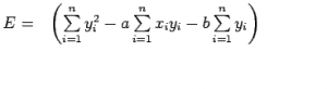
Now consider the sum of the squares of ei
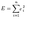
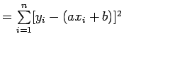
Note: E is a function of parameters a and b and we need to find a and b such that E is minimum and the necessary condition for E to be minimum is as follows:

This condition yields:
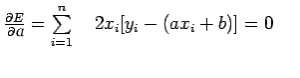
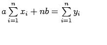
Above two equations are called normal equation which are solved to get the value of a and b.
The Expression for E can be rewritten as:
The basic syntax for a regression analysis in R is
lm(Y ~ model)
where Y is the object containing the dependent variable to be predicted and model is the formula for the chosen mathematical model.
The command lm( ) provides the model’s coefficients but no further statistical information.
Following R code is used to implement SIMPLE LINEAR REGRESSION:
# Simple Linear Regression
# Importing the dataset
dataset = read.csv('salary.csv')
# Splitting the dataset into the
# Training set and Test set
install.packages('caTools')
library(caTools)
split = sample.split(dataset$Salary, SplitRatio = 0.7)
trainingset = subset(dataset, split == TRUE)
testset = subset(dataset, split == FALSE)
# Fitting Simple Linear Regression to the Training set
lm.r= lm(formula = Salary ~ YearsExperience,
data = trainingset)
coef(lm.r)
# Predicting the Test set results
ypred = predict(lm.r, newdata = testset)
install.packages("ggplot2")
library(ggplot2)
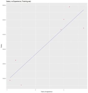
# Visualising the Training set results
ggplot() + geom_point(aes(x = trainingset$YearsExperience,
y = trainingset$Salary), colour = 'red') +
geom_line(aes(x = trainingset$YearsExperience,
y = predict(lm.r, newdata = trainingset)), colour = 'blue') +
ggtitle('Salary vs Experience (Training set)') +
xlab('Years of experience') +
ylab('Salary')
# Visualising the Test set results
ggplot() +
geom_point(aes(x = testset$YearsExperience, y = testset$Salary),
colour = 'red') +
geom_line(aes(x = trainingset$YearsExperience,
y = predict(lm.r, newdata = trainingset)),
colour = 'blue') +
ggtitle('Salary vs Experience (Test set)') +
xlab('Years of experience') +
ylab('Salary')
Output of coef(lm.r):
Intercept YearsExperience
24558.39 10639.23
Visualising the Training set results:
Visualising the Testing set results:
