")
Univariate data is the type of data in which the result depends only on one variable. For instance, dataset of points on a line can be considered as a univariate data where abscissa can be considered as input feature and ordinate can be considered as output/result.
For example:
For line Y = 2X + 3;
Input feature will be X and Y will be the result.
X Y
1 5
2 7
3 9
4 11
5 13
Concept:
For univariate linear regression, there is only one input feature vector. The line of regression will be in the form of:
Y = b0 + b1 * X
Where,
b0 and b1 are the coefficients of regression.
Hence, it is being tried to predict regression coefficients b0 and b1 by training a model.
Utility functions
Predict
def predict(x, b0, b1):
"""Predicts the value of prediction based on
current value of regression coefficients when input is x"""
# Y = b0 + b1 * X
return b0 + b1 * x
Cost function :
Cost function computes the error percentage with the current value of regression coefficients. It quantitatively defines how far the model is wrt actual regression coefficients which has lowest rate of error.
def cost(x, y, b0, b1):
# y is a list of expected value
errors = []
for x, y in zip(x, y):
prediction = predict(x, b0, b1)
expected = y
difference = prediction-expected
errors.append(difference)
# Now, we have errors for all the observations,
# for some input, the value of error might be positive
# and for some input might be negative,
# and if we directly add them up,
# the values might cancel out leading to wrong output."
# Hence, we use concept of mean squared error.
# in mse, we return mean of square of all the errors.
mse = sum([e * e for e in errors])/len(errors)
return mse
Cost Derivative
After each iteration, the cost is upgraded in proportion to the error. The nature of error is very data sensitive. By data sensitive i mean the error value changes very fast, because we had square in error function. Hence, to make it more tolerant to high values of errors, we derivate the error function.
The mathematics is as follows:
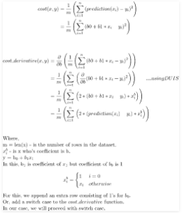
Code:
def cost_derivative(x, y, b0, b1, i):
return sum([
2*(predict(xi, b0, b1)-yi)*1
if i == 0
else 2*(predict(xi, b0, b1)-yi)*xi
for xi, yi in zip(x, y)
])/len(x)
Update Coefficients :
At each iteration (epoch), the values of the regression coefficient are updated by a specific value wrt to the error from the previous iteration. This updation is very crucial and is the crux of the machine learning applications that you write.
Updating the coefficients with exact an update of a coefficient is done by penalizing its value with a fraction of error that it’s previous values caused.
This fraction is called as learning rate. This defines how fast our model reaches out to point of convergence(point where error is ideally 0).

Python function for the same is as follows:
def update_coeff(x, y, b0, b1, i, alpha):
bi -= alpha * cost_derivative(x, y, b0, b1, i)
return bi
Stop Iterations:
This is the function which is used to specify when should the iterations should stop.
As per user, the algorithm stop_iteration generally returns true in following conditions:
Max Iteration : Model is trained for a specified number of iterations.
Error value : Depending upon the value of previous error, the algorithm decides whether to continue or stop.
Accuracy : Depending upon the last accuracy of the model, if it is larger than the mentioned accuracy, the algorithm returns True,
Hybrid : This is more often used. This combines more than one above mentioned conditions along with an exceptional break option. Exceptional break is condition where training continues until when something bad happens. Something bad might include overflow of result, time constraints exceeded, etc.
Having all the utility functions defined, lets see the pseudo code followed by its implementation:
Code :
x, y is the given data.
(b0, b1) <-- (0, 0)
i = 0
while True:
if stop_iteration(i):
break
else:
b0 = update_coeff(x, y, b0, b1, 0, alpha)
b1 = update_coeff(x, y, b0, b1, 1, alpha)
Final Oop implementation :
class LinearRegressor:
def __init__(self, x, y, alpha = 0.01, b0 = 0, b1 = 0):
"""
x: input feature
y: result / target
alpha: learning rate, default is 0.01
b0, b1: linear regression coefficient.
"""
self.i = 0
self.x = x
self.y = y
self.alpha = alpha
self.b0 = b0
self.b1 = b1
if len(x) != len(y):
raise TypeError("x and y should have same number of rows.")
def predict(model, x):
"""Predicts the value of prediction based on
current value of regression coefficients when input is x"""
# Y = b0 + b1 * X
return model.b0 + model.b1 * x
def cost_derivative(model, i):
x, y, b0, b1 = model.x, model.y, model.b0, model.b1
predict = model.predict
return sum([
2 * (predict(xi) - yi) * 1
if i == 0
else (predict(xi) - yi) * xi
for xi, yi in zip(x, y)
]) / len(x)
def update_coeff(model, i):
cost_derivative = model.cost_derivative
if i == 0:
model.b0 -= model.alpha * cost_derivative(i)
elif i == 1:
model.b1 -= model.alpha * cost_derivative(i)
def stop_iteration(model, max_epochs = 1000):
model.i += 1
if model.i == max_epochs:
return True
else:
return False
def fit(model):
update_coeff = model.update_coeff
model.i = 0
while True:
if model.stop_iteration():
break
else:
update_coeff(0)
update_coeff(1)
if __name__ == '__main__':
linearRegressor = LinearRegressor(
x =[i for i in range(12)],
y =[2 * i + 3 for i in range(12)],
alpha = 0.03
)
linearRegressor.fit()
print(linearRegressor.predict(12))
# expects 2 * 12 + 3 = 27