")
This article discusses the basics of Softmax Regression and its implementation in Python using TensorFlow library.
What is Softmax Regression?
Softmax regression (or multinomial logistic regression) is a generalization of logistic regression to the case where we want to handle multiple classes.
A gentle introduction to linear regression can be found here:
Understanding Logistic Regression
In binary logistic regression we assumed that the labels were binary, i.e. for i^{th} observation,
y_{i} epsilon begin{Bmatrix} 0, 1 end{Bmatrix}
But consider a scenario where we need to classify an observation out of two or more class labels. For example, digit classification. Here, the possible labels are:
y_{i} epsilon begin{Bmatrix} 0, 1, 2, 3, 4, 5, 6, 7, 8, 9 end{Bmatrix}
In such cases, we can use Softmax Regression.
Let us first define our model:
- Let the dataset have ‘m’ features and ‘n’ observations. Also, there are ‘k’ class labels, i.e every observation can be classified as one of the ‘k’ possible target values. For example, if we have a dataset of 100 handwritten digit images of vector size 28×28 for digit classification, we have, n = 100, m = 28×28 = 784 and k = 10.
- Feature matrix
The feature matrix, X, is represented as:Here, x_{ij} denotes the values of j^{th} feature for i^{th} observation. The matrix has dimensions: nspace X space (m+1) - Weight matrix
We define a weight matrix, W as:Here, w_{ij} represents the weight assigned to i^{th} feature for j^{th} class label. The matrix has dimensions:(m+1)space X space k. Initially, weight matrix is filled using some normal distribution. - Logit score matrix
Then, we define our net input matrix(also called logit score matrix), Z, as:The matrix has dimensions: n space X space k.
Currently, we are taking an extra column in feature matrix, X and an extra row in weight matrix, W. These extra columns and rows correspond to the bias terms associated with each prediction. This could be simplified by defining an extra matrix for bias, b of size n space X space k where b_{ij} = w_{0j}. (In practice, all we need is a vector of size k and some broadcasting techniques for the bias terms!)
So, the final score matrix, Z is:
where X matrix has dimensions nspace X space m while W has dimensions mspace X space k. But Z matrix still has same value and dimensions!
But what does matrix Z signify? Actually, Z_{ij} is the likelihood of label j for i^{th} observation. It is not a proper probability value but can be considered as a score given to each class label for each observation!
Let us define Z_i as the logit score vector for i^{th} observation.
For example, let the vector Z_5 = [1.1, 2.0, 3.1, 5.2, 1.0, 1.5, 0.2, 0.1, 1.2, 0.4] represents the score for each of the class labels {0,1,2,3,4,5,6,7,8,9} in handwritten digit classification problem for 5^{th} observation. Here, the max score is 5.2 which corresponds to class label ‘3’. Hence, our model currently predicts the 5^{th} observation/image as ‘3’.
Softmax layer
It is harder to train the model using score values since it is hard to differentiate them while implementing Gradient Descent algorithm for minimizing the cost function. So, we need some function which normalizes the logit scores as well as makes them easily differentiable!In order to convert the score matrix Z to probabilities, we use Softmax function.
For a vector y, softmax function S(y) is defined as:
So, softmax function will do 2 things:
1. convert all scores to probabilities.
2. sum of all probabilities is 1.
Recall that in Binary Logistic classifier, we used sigmoid function for the same task. Softmax function is nothing but a generalization of sigmoid function! Now, this softmax function computes the probability that the i^{th} training sample belongs to class j given the logits vector Z_i as:
In vector form, we can simply write:
For simplicity, let S_i denote the softmax probability vector for i^{th} observation.
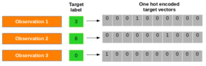
- One-hot encoded target matrix
Since softmax function provides us with a vector of probabilities of each class label for a given observation, we need to convert target vector in the same format to calculate the cost function! Corresponding to each observation, there is a target vector (instead of a target value!) composed of only zeros and ones where only correct label is set as 1. This technique is called one-hot encoding.See the diagram given below for a better understanding:
Now, we denote one-hot encoding vector for i^{th} observation as T_i
Cost function
Now, we need to define a cost function for which, we have to compare the softmax probabilities and one-hot encoded target vector for similarity. We use the concept of Cross-Entropy for the same. The Cross-entropy is a distance calculation function which takes the calculated probabilities from softmax function and the created one-hot-encoding matrix to calculate the distance. For the right target classes, the distance values will be lesser, and the distance values will be larger for the wrong target classes.We define cross entropy, D(S_i,T_i) for i^{th} observation with softmax probability vector, S_i and one-hot target vector, T_i as:
And now, cost function, J can be defined as the average cross entropy, i.e:
and the task is to minimize this cost function!
Gradient Descent algorithm
In order to learn our softmax model via gradient descent, we need to compute the derivative:
and
which we then use to update the weights and biases in opposite direction of the gradient:
and
for each class j where j in {1,2,..,k} and alpha is learning rate.Using this cost gradient, we iteratively update the weight matrix until we reach a specified number of epochs (passes over the training set) or reach the desired cost threshold.
Implementation
Let us now implement Softmax Regression on the MNIST handwritten digit dataset using TensorFlow library.
For a gentle introduction to TensorFlow, follow this tutorial:
Introduction to TensorFlow
Step 1: Import the dependencies
First of all, we import the dependencies.
import tensorflow as tf
import numpy as np
import matplotlib.pyplot as plt
Step 2: Download the data
TensorFlow allows you to download and read in the MNIST data automatically. Consider the code given below. It will download and save data to the folder, MNIST_data, in your current project directory and load it in current program.
from tensorflow.examples.tutorials.mnist import input_data
mnist = input_data.read_data_sets("MNIST_data/", one_hot=True)
Extracting MNIST_data/train-images-idx3-ubyte.gz
Extracting MNIST_data/train-labels-idx1-ubyte.gz
Extracting MNIST_data/t10k-images-idx3-ubyte.gz
Extracting MNIST_data/t10k-labels-idx1-ubyte.gz
Step 3: Understanding data
Now, we try to understand the structure of the dataset.
The MNIST data is split into three parts: 55,000 data points of training data (mnist.train), 10,000 points of test data (mnist.test), and 5,000 points of validation data (mnist.validation).
Each image is 28 pixels by 28 pixels which has been flattened into 1-D numpy array of size 784. Number of class labels is 10. Each target label is already provided in one-hot encoded form.
print("Shape of feature matrix:", mnist.train.images.shape)
print("Shape of target matrix:", mnist.train.labels.shape)
print("One-hot encoding for 1st observation:n", mnist.train.labels[0])
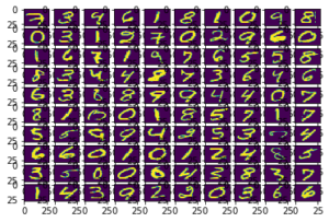
# visualize data by plotting images
fig,ax = plt.subplots(10,10)
k = 0
for i in range(10):
for j in range(10):
ax[i][j].imshow(mnist.train.images[k].reshape(28,28), aspect='auto')
k += 1
plt.show()
Output:
Shape of feature matrix: (55000, 784)
Shape of target matrix: (55000, 10)
One-hot encoding for 1st observation:
[ 0. 0. 0. 0. 0. 0. 0. 1. 0. 0.]
Step 4: Defining computation graph
Now, we create a computation graph.
# number of features
num_features = 784
# number of target labels
num_labels = 10
# learning rate (alpha)
learning_rate = 0.05
# batch size
batch_size = 128
# number of epochs
num_steps = 5001
# input data
train_dataset = mnist.train.images
train_labels = mnist.train.labels
test_dataset = mnist.test.images
test_labels = mnist.test.labels
valid_dataset = mnist.validation.images
valid_labels = mnist.validation.labels
# initialize a tensorflow graph
graph = tf.Graph()
with graph.as_default():
"""
defining all the nodes
"""
# Inputs
tf_train_dataset = tf.placeholder(tf.float32, shape=(batch_size, num_features))
tf_train_labels = tf.placeholder(tf.float32, shape=(batch_size, num_labels))
tf_valid_dataset = tf.constant(valid_dataset)
tf_test_dataset = tf.constant(test_dataset)
# Variables.
weights = tf.Variable(tf.truncated_normal([num_features, num_labels]))
biases = tf.Variable(tf.zeros([num_labels]))
# Training computation.
logits = tf.matmul(tf_train_dataset, weights) + biases
loss = tf.reduce_mean(tf.nn.softmax_cross_entropy_with_logits(
labels=tf_train_labels, logits=logits))
# Optimizer.
optimizer = tf.train.GradientDescentOptimizer(learning_rate).minimize(loss)
# Predictions for the training, validation, and test data.
train_prediction = tf.nn.softmax(logits)
valid_prediction = tf.nn.softmax(tf.matmul(tf_valid_dataset, weights) + biases)
test_prediction = tf.nn.softmax(tf.matmul(tf_test_dataset, weights) + biases)
Some important points to note:
For the training data, we use a placeholder that will be fed at run time with a training minibatch. The technique of using minibatches for training model using gradient descent is termed as Stochastic Gradient Descent.
In both gradient descent (GD) and stochastic gradient descent (SGD), you update a set of parameters in an iterative manner to minimize an error function. While in GD, you have to run through ALL the samples in your training set to do a single update for a parameter in a particular iteration, in SGD, on the other hand, you use ONLY ONE or SUBSET of training sample from your training set to do the update for a parameter in a particular iteration. If you use SUBSET, it is called Minibatch Stochastic gradient Descent. Thus, if the number of training samples are large, in fact very large, then using gradient descent may take too long because in every iteration when you are updating the values of the parameters, you are running through the complete training set. On the other hand, using SGD will be faster because you use only one training sample and it starts improving itself right away from the first sample. SGD often converges much faster compared to GD but the error function is not as well minimized as in the case of GD. Often in most cases, the close approximation that you get in SGD for the parameter values are enough because they reach the optimal values and keep oscillating there.
The weight matrix is initialized using random values following a (truncated) normal distribution. This is achieved using tf.truncated_normal method. The biases get initialized to zero using tf.zeros method.
Now, we multiply the inputs with the weight matrix, and add biases. We compute the softmax and cross-entropy using tf.nn.softmax_cross_entropy_with_logits (it’s one operation in TensorFlow, because it’s very common, and it can be optimized). We take the average of this cross-entropy across all training examples using tf.reduce_mean method.
We are going to minimize the loss using gradient descent. For this, we use tf.train.GradientDescentOptimizer.
train_prediction, valid_prediction and test_prediction are not part of training, but merely here so that we can report accuracy figures as we train.
Step 5: Running the computation graph
Since we have already built the computation graph, now it’s time to run it through a session.
# utility function to calculate accuracy
def accuracy(predictions, labels):
correctlY_predictionicted = np.sum(np.argmax(predictions, 1) == np.argmax(labels, 1))
accu = (100.0 * correctlY_predictionicted) / predictions.shape[0]
return accu
with tf.Session(graph=graph) as session:
# initialize weights and biases
tf.global_variables_initializer().run()
print("Initialized")
for step in range(num_steps):
# pick a randomized offset
offset = np.random.randint(0, train_labels.shape[0] - batch_size - 1)
# Generate a minibatch.
batch_data = train_dataset[offset:(offset + batch_size), :]
batch_labels = train_labels[offset:(offset + batch_size), :]
# Prepare the feed dict
feed_dict = {tf_train_dataset : batch_data,
tf_train_labels : batch_labels}
# run one step of computation
_, l, predictions = session.run([optimizer, loss, train_prediction],
feed_dict=feed_dict)
if (step % 500 == 0):
print("Minibatch loss at step {0}: {1}".format(step, l))
print("Minibatch accuracy: {:.1f}%".format(
accuracy(predictions, batch_labels)))
print("Validation accuracy: {:.1f}%".format(
accuracy(valid_prediction.eval(), valid_labels)))
print("nTest accuracy: {:.1f}%".format(
accuracy(test_prediction.eval(), test_labels)))
Output:
Initialized
Minibatch loss at step 0: 11.68728256225586
Minibatch accuracy: 10.2%
Validation accuracy: 14.3%
Minibatch loss at step 500: 2.239773750305176
Minibatch accuracy: 46.9%
Validation accuracy: 67.6%
Minibatch loss at step 1000: 1.0917563438415527
Minibatch accuracy: 78.1%
Validation accuracy: 75.0%
Minibatch loss at step 1500: 0.6598564386367798
Minibatch accuracy: 78.9%
Validation accuracy: 78.6%
Minibatch loss at step 2000: 0.24766433238983154
Minibatch accuracy: 91.4%
Validation accuracy: 81.0%
Minibatch loss at step 2500: 0.6181786060333252
Minibatch accuracy: 84.4%
Validation accuracy: 82.5%
Minibatch loss at step 3000: 0.9605385065078735
Minibatch accuracy: 85.2%
Validation accuracy: 83.9%
Minibatch loss at step 3500: 0.6315320730209351
Minibatch accuracy: 85.2%
Validation accuracy: 84.4%
Minibatch loss at step 4000: 0.812285840511322
Minibatch accuracy: 82.8%
Validation accuracy: 85.0%
Minibatch loss at step 4500: 0.5949224233627319
Minibatch accuracy: 80.5%
Validation accuracy: 85.6%
Minibatch loss at step 5000: 0.47554320096969604
Minibatch accuracy: 89.1%
Validation accuracy: 86.2%
Test accuracy: 86.5%
Some important points to note:
In every iteration, a minibatch is selected by choosing a random offset value using np.random.randint method.
To feed the placeholders tf_train_dataset and tf_train_label, we create a feed_dict like this:
feed_dict = {tf_train_dataset : batch_data, tf_train_labels : batch_labels}
A shortcut way of performing one step of computation is:
_, l, predictions = session.run([optimizer, loss, train_prediction], feed_dict=feed_dict)
This node returns the new values of loss and predictions after performing optimization step.
This brings us to the end of the implementation. Complete code can be found here.
Finally, here are some points to ponder upon:
You can try to tweak with the parameters like learning rate, batch size, number of epochs, etc and achieve better results. You can also try a different optimizer like tf.train.AdamOptimizer.
Accuracy of above model can be improved by using a neural network with one or more hidden layers. We will discuss its implementation using TensorFlow in some upcoming articles.
Softmax Regression vs. k Binary Classifiers
One should be aware of the scenarios where softmax regression works and where it doesn’t. In many cases, you may need to use k different binary logistic classifiers for each of the k possible values of the class label.
Suppose you are working on a computer vision problem where you’re trying to classify images into three different classes:
Case 1: Suppose that your classes are indoor_scene, outdoor_urban_scene, and outdoor_wilderness_scene.
Case 2: Suppose your classes are indoor_scene, black_and_white_image, and image_has_people.
In which case you would use Softmax Regression classifier and in which case you would use 3 Binary Logistic Regression classifiers?
This will depend on whether the 3 classes are mutually exclusive.
In case 1, a scene can be either indoor_scene, outdoor_urban_scene or outdoor_wilderness_scene. So, assuming that each training example is labeled with exactly one of the 3 classes, we should build a softmax classifier with k = 3.
However, in case 2, the classes are not mutually exclusive since a scene can be both indoor and have people in it. So, in this case, it would be more appropriate to build 3 binary logistic regression classifiers. This way, for each new scene, your algorithm can separately decide whether it falls into each of the 3 categories.